Hello world (again and again)

For the past 20 years or so, I’ve used the image you see in the upper left of this site as an avatar icon. People have asked about it over the years, and usually they reference feathers, or topographical maps, or a cresting ocean wave. It does visually reference all of these things, but its true origin is a crop of an image I made early in graduate school, when I was learning about dynamical systems.

I remember working through Strogatz’s classic Nonlinear Dynamics and Chaos in 2006–2007, front to back, reading it on the way home from lab, taking the Green line to Lechmere. That book changed the way I looked (look) at the world in a way only a few others have. I’d taken calculus and differential equations in college, but in a practical sense, analytical approaches seemed… too hard. Hard and relatively limited. The major insights that clicked from the book were 1) the breadth of things that could be described in terms of interdependent rates of change was essentially endless and 2) studying the dynamics of the evolution of these systems could give you intuition and insight even if you didn’t (or couldn’t!) solve the equations directly. Even better, there was a computational toolset that I could use to capture the essentials of problems and study them: numerical integration.

I saved the image, but over the years I’d forgotten the software I used to generate it. When I started this post, I was doubtful I could ever find it, but I did — it was XPPAUT/XPP. Written by Bard Ermentrout, it’s still online! The site’s aesthetic is clearly “of a time”, but remarkably, it’s still up-to-date and they even have a build for Apple Silicon. Respect. XPPAUT is remarkably full-featured and a powerful learning tool; I’m probably one of many who have benefited from it over the years.

The system I was exploring was the Morris-Lecar model, developed by Catherine Morris and Harold Lecar when they were at the NIH in their 1981 paper “Voltage Oscillations in the Barnacle Giant Muscle Fiber”. It came out within a month of when I was born. This model is part of a long lineage of mathematical neuroscience that started with Hodgkin and Huxley’s work on the squid giant axon (a tremendous and prescient achievement for which they won the Nobel in 1963). Quoting Morris and Lecar’s abstract:

Barnacle muscle fibers subjected to constant current stimulation produce a variety of types of oscillatory behavior … This paper presents an analysis of the possible modes of behavior available to a system of two noninactivating conductance mechanisms, and indicates a good correspondence to the types of behavior exhibited by barnacle fiber.

A (relatively) simple model for a (relatively) simple neuron, but a lot of great lessons to be had.

Background on the Morris-Lecar equations

At a high level, the system can be described by two interdependent variables that change over time, $V$ and $N$. Everything else below just shapes the core dynamics. The following two equations describe how they change over time:

$$C\frac{dV}{dt} = I - g_L(V - V_L) - g_{Ca}\,M_{ss}(V - V_{Ca}) - g_K\,N(V - V_K)$$ $$\frac{dN}{dt} = \frac{N_{ss} - N}{\tau_N}$$

where

$$M_{ss} = \frac{1}{2}\left(1 + \tanh\frac{V - V_1}{V_2}\right)$$ $$N_{ss} = \frac{1}{2}\left(1 + \tanh\frac{V - V_3}{V_4}\right)$$ $$\tau_N = \frac{1}{\varphi\,\cosh\!\left(\frac{V - V_3}{2V_4}\right)}$$

Variables

• $V$: membrane potential
• $N$: recovery variable — the probability that the K⁺ channel is conducting
• $I$: applied current
• $C$: membrane capacitance
• $g_L$, $g_{Ca}$, $g_K$: leak, Ca²⁺, and K⁺ conductances through membrane channels
• $V_L$, $V_{Ca}$, $V_K$: equilibrium potential of relevant ion channels
• $V_1$, $V_2$, $V_3$, $V_4$: tuning parameters for steady state and time constant
• $\varphi$: reference frequency

$V$ — this is the overall voltage of the system. At rest, neurons pump ions across their cell membrane such that there is a stereotypical voltage difference (different in every type of neuron). Each ion has its own equilibrium set point, where the concentration gradient is perfectly counterbalanced by the charge gradient. The voltage difference across the membrane at any given time is a dynamic weighted average of all the equilibria in the system. The weights are given by the probability that ion channels of that type are open. The beautiful thing about electrophysiology is that the probability of ion channel opening depends on the voltage, and when they open, they change the voltage. This feedback means that depending on the specific relationship between open probability and voltage, and to what degree the equilibria of the ions are positive or negative, you can have many different types of system behaviors.

The change in $V$ is proportional to the sum of all currents in the system: an artificially applied current ($I$), and the currents of Ca²⁺, K⁺, and a generic “leak” current ($L$). The amplitude of these ionic currents is proportional to how far the membrane voltage is from their respective equilibria. (In particular, note how the K⁺ current depends on $N$.)

$N$ — this is a “recovery variable”, and reflects the probability that a K⁺ channel (which will drive the system to rest) is open. The change in $N$ is proportional to the difference from its steady-state value, which is in turn a function of $V$.

These two variables are sufficient to describe the state of the system, and if you plot them against each other over time, you get what is known as a phase diagram. If you plot just $V$ over time, you can see the “activity” of the neuron.

I wrote my own simulation of this system to make both of those types of plots, for various conditions. I’d suggest you poke around and come back.

Explorations

The amazing thing about this system is that it is bistable. If you track the dynamics of $V$ and $N$ over time, there are two types of qualitative behavior that you can observe: fixed point and limit cycle.

Fixed point — for our default conditions, this happens when there is no applied current ($I_{app} = 0$). The system is at rest and stays at rest. Small perturbations will just evolve back to the starting point in the phase diagram. A screenshot here wouldn’t be terribly dynamic, so I’d just suggest exploring by clicking around.

Explore fixed point dynamics →

Limit cycle — Given enough stimulation, however, something very different happens. The voltage creeps up and then quickly shoots towards and past 0 mV as the Ca²⁺ channels open. The system doesn’t stay there. Other ion channels that open only at high voltage (K⁺) start to conduct, which drives the voltage back down — the system has built-in negative feedback. The remarkable thing is that this is not enough to get the system to reset because of the continual stimulus. Over time, the K⁺ channels trade off with the Ca²⁺ channels, which push the system back up, again and again.

Explore the limit cycle →

Here’s a figure with a trace of this behavior in both phase and voltage plots:

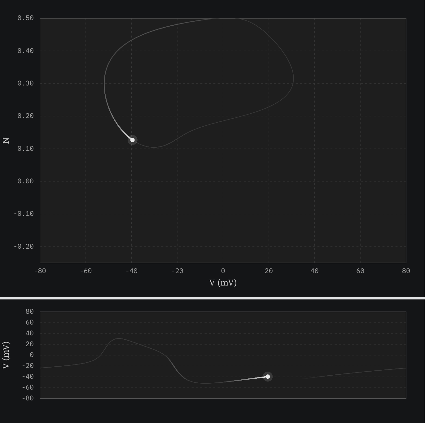
This is sort of like an infinite roller coaster loop where the engine turns on at the bottom of the loop and off at the top, where gravity takes over. As long as the coaster is going fast enough to get up to the top of the loop, the engine will kick in enough at the bottom to continue looping.

The avatar, revisited

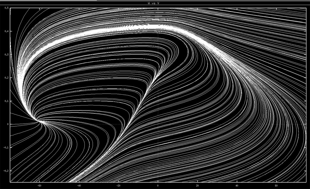
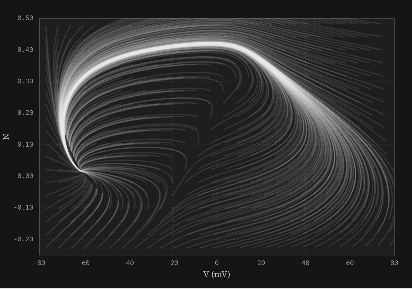
So, anyway, where does the original image come from? One way to understand a phase diagram is to seed a bunch of starting conditions at once, and let them all play out. If you do this with no applied current in my simulator, you re-create the figure I made almost twenty years ago.

It’s fun to visualize the bifurcation in the system in this mode by adjusting the current ($I$).

Explore the flow field →

The swooping lines all converge on the fixed point, and many (most?) of them ride the limit cycle groove on the way back. This picture is akin to letting 100 balls roll down a hill, starting at different points up the slope, or tracing every droplet of a wave as it crashes. The ridge in the middle that is part of the crop illustrates the threshold between the fixed point and limit cycle behavior.

I’ve used this as my avatar for many years. Recreating it for this post, I love it just as much now as I did then. We are surrounded by twirling, converging elegance, even within something as simple as a barnacle. The same math used here can also capture phenomena like predator-prey cycles, firefly synchronization, and the feedback loops that generate circadian rhythms. It touches on a profound universality. My career has diverged from neuroscience, but I’ve kept the avatar as a reminder of what it feels like to see the world this way.